As much as physics simulation is a bottleneck to better engineering, so too is human imagination. To build beyond, our researchers have created a foundation model for geometry that understands how any 3D shape relates to any other, and knows what lies between an aircraft wing and a feathered bird’s wing.
Our latest Large Geometry Model, LGM-Aero, has 100M parameters (approximately as many as OpenAI’s GPT1) and has seen 25M diverse 3D shapes. Our foundation model has already been deployed in real-world customer challenges, outperforming current state-of-the art engineering workflows.
In previous posts we gave an executive overview of the implications of LGM-Aero for engineering and unveiled Ai.rplane, a public-facing reference application that allows anyone to design their own aircraft, powered by LGM-Aero.
In this post, we explore the capabilities of our new model and delve into its architecture and development. We will release a full technical paper with benchmarks soon.
Why do we need foundation models in engineering?
The typical process for engineering physical parts starts with engineers using computer aided design (CAD) to create a precise digital schematic of the part, often with tuneable parameters such as the length of a wing or the size of an inlet. The CAD software then outputs an explicit representation (called a mesh) of the geometry, comprising vertices joined by faces. The mesh is then fed into numerical simulations – such as computational fluid dynamics (CFD) or finite element analysis (FEA) – that are used to estimate the performance characteristics of the design, allowing engineers to understand how their components would perform in the real world and identify potential issues without needing to build physical prototypes.
Engineers then iterate on the design by tuning the parameters based on the insights they gain from simulations. This process usually involves multiple rounds of testing and refinement to reach the necessary performance, requiring hundreds of hours of waiting for simulation results and months of iteration time.
With a foundation model of geometry we are setting out to endogenize the full description of the shape of an object and so make it subject to an optimization process - rather than a small number of ex ante defined parameters pertaining to some starting shape.
1. Constructing representations of geometry for prediction and optimisation
To train a machine learning model that can predict the performance characteristics of a design - unlocking design optimization due to the rapid inference speed of machine learning models over traditional simulation - we require a representation of the design that can be input to a machine learning model.
The obvious choice is to train a traditional machine learning algorithm directly on the value of the parameters used by the CAD to generate the mesh. Unfortunately, this suffers from a number of issues:
- a CAD parametrisation is specific to one class of designs for a single object - there is no way to tweak the parameters of a CAD representation of an aircraft to make it produce a banana - preventing predictive models trained on CAD parameters from generalising across different CAD parameterisations; and,
- CAD similarity can have little to do with geometric similarity — designs with similar CAD parameters may correspond to very different geometric objects in physical space.
An alternative is to use a machine learning model that can ingest the mesh generated by the CAD, but that comes with its own set of issues:
- meshes require sophisticated models that can deal with their large graph structure and that do not require a fixed-size representation for every geometric object, as a mesh for one geometry might require many more vertices than for another;
- meshes, while they respect physical similarity as they explicitly represent shapes, are not unique representations of the underlying smooth geometries; and,
- meshes are very high-dimensional objects, so traditional optimization methods often struggle to break free from local optima, limiting the exploration of novel design spaces.
Our foundation model offers a solution by compressing the essence of any geometry into a vector of size 512, a size universally shared across all geometries. This unlocks efficient downstream models for predicting performance for a given design, and also offers a natural solution space for optimizers to explore. Our methods can then rapidly generate and explore diverse design options across the Pareto front, the space of optimal tradeoffs among competing objectives.
This empowers engineers to consider a broader range of optimal solutions, balancing multiple factors such as weight, strength, and performance. Engineers can then easily iterate their performance requirements, finding the best design in minutes, rather than weeks.
2. Overcoming data scarcity with transfer learning
Numerical simulation data can be slow and costly to produce, often requiring significant time and compute to generate accurate results. While our advanced active learning techniques have significantly reduced data requirements, foundation models allow us to take this a step further.
A key advantage of our geometry foundation model is its ability to deliver benefits across a spectrum of data availability scenarios. For companies with extensive data assets, the model can be fine-tuned to enhance performance in specific areas of interest and provide transfer learning across related tasks. This enables organizations to create new value from the numerical simulations used in the development of historical designs.
Importantly, our foundation model is designed to provide significant advantages even for organizations with limited historical data. The pre-trained model can deliver instant benefits out of the box, often outperforming traditional methods, without the need for extensive fine-tuning. This accessibility means that companies with few samples can still leverage the power of AI to improve their design processes and outcomes.
The versatility of our foundation model in handling both data-rich and data-scarce scenarios represents a significant leap forward in engineering design. It offers the potential to overcome longstanding bottlenecks, reduce development times, and unlock new realms of design possibilities for organizations of different sizes and data capacities.
3. Discovering novel designs
The greatest performance gains often come from complete redesigns of a part, rather than from tuning a few aspects of an existing design. By optimizing designs with a foundation model that has been exposed to millions of geometries, we unlock novel optimization directions - a generative model trained solely on traditional aircraft cannot produce biplanes, but a generative foundation model can discover them.
By unlocking design optimization through the space of all geometry, our foundation model for geometry frees engineers to focus on the performance of the entire system, rather than obsessing over the shape of an individual part.
Unlocking real-world impact
While the theoretical benefits of foundation models are compelling, their real-world impact is what really matters. We have begun deploying our foundation model with clients on a range of problems, yielding impressive results. A recent example is our collaboration with a major European automotive manufacturer.
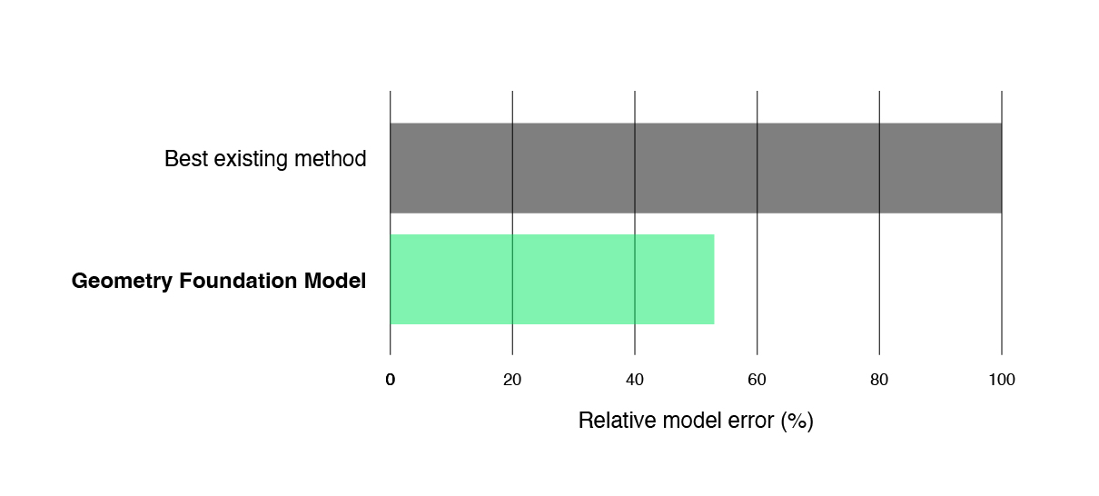
Optimal airflow around cars is critical to cooling, aerodynamics, and reducing system costs. Our foundation model, without any fine-tuning or active learning, surpassed the existing optimized design of a car component within minutes. It achieved a remarkable 7% increase in aerodynamic performance alongside a 10% reduction in mass when compared to the current best design. With regards to accuracy, the predictive tasks on the foundation model’s representations are more accurate than the same predictive tasks applied directly to CAD parameters – highlighting how our geometry foundation model is successful at representing geometry efficiently and usefully.
Under the hood: a schematic of LGM-Aero
Our foundation model captures the essence of a surface design in a list of 512 numbers. By mapping designs to this list we gain a highly-compact representation that can be used with any of the classic machine learning techniques to predict design performance, while by mapping from a new list we can create novel designs beyond human imagination.
Our geometric foundation model is a coupling of two parts:
- An encoder that looks at the triangular mesh describing a surface and predicts a list of 512 numbers that capture the essence of how that surface is different from other surfaces. We call that list of numbers the latent code.
- A decoder that looks at the latent code and learns to predict how far away any given point in 3D space is from the surface corresponding to that latent code, as well as whether that point is inside or outside that surface. Points whose distance from the surface is exactly zero lie on the surface, meaning that the decoder implicitly predicts where the surface lies.
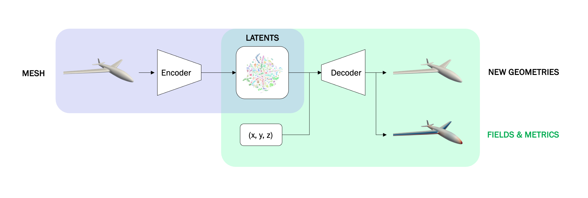
We “capture the essence” of geometry by training these two parts in tandem, end-to-end: the encoder has predicted a good latent code for a surface if the decoder is able to exactly predict the relationship between points in 3D space and the surface.
The decoder’s job is made easiest if a small change to the latent code (say, adding 0.001 to one of the 512 numbers) causes a correspondingly small change in the 3D surface predicted by the decoder. By making a series of such small changes we should be able to accumulate these small changes in the surface into a large change – we can smoothly walk through latent space (the 512-dimensional space in which latent codes live) between any two shapes. In other words, we can take an aircraft and morph it into a goshawk.
The middle panel of the video below is a 2D projection of the 512-dimensional latent space (much like how a flat map of the world is a 2D projection of the 3D globe). The points are the locations of several thousand flying objects. The black point traces out a path through latent space, with the left panel showing the surface corresponding to the current point. As we will discuss below and is shown in the right panel, the latent code can be decoded to predict physics as well as geometry.
Whilst trained together, the encoder and decoder are independently useful.
Encoder
Suppose we want to train a machine learning model on a dataset of aircraft and measurements of their lift-over-drag coefficient (how many metres the plane moves horizontally vs how many metres it falls vertically) to predict how well a new aircraft design will fly. Conventionally, this would require reaching for a geometric deep learning architecture (such as the one we used in our encoder), which can be fiddly to set-up and expensive to train. With our pre-trained encoder you circumvent this difficulty: the encoder converts each of your aircraft into a list of 512 numbers, which can straightforwardly be used as the features to train any classical model (linear regression, neural network, random forest, gradient boosted decision trees, etc.). We have had particular success using Gaussian Processes to predict the engineering performance of novel designs, because the predictive uncertainty can be used in an active learning loop to trigger new simulations when a novel design is so far from the human-imagined designs that the predictions are no longer accurate.
Decoder
We can use the decoder to generate a novel design by picking a latent code and extracting the surface, bypassing the need for computer-aided design (CAD). What’s even better is that we can optimize: starting from a random latent code, we can make a series of iterative small changes to that latent code to make the corresponding surface obey constraints and improve objectives (gradient-based optimization). Another application is predicting physics associated with geometry. Having already trained the decoder to predict one function of 3D coordinate (distance from surface), we can train it to predict others, such as the flow of air around an aircraft or the pressure on its surface.
In the right-hand panel of the movie above we illustrate both of these use cases. The slider at the bottom shows a prediction of the drag from a Gaussian Process trained on the latent codes, while the colours on the surface show pressure predictions from a fine-tuned decoder.
NB: Gaussian Process was a modelling choice here, but any other standard model can be used for prediction, like random forests, neural networks, or even linear regression. Of course, some models will be more or less suitable for the task at hand, but the point is that the whole arsenal of traditional ML can be brought to bear on downstream problems. This unshackles practitioners from more cumbersome models, like graph neural networks, that are required to ingest and predict on geometric objects.
How we trained LGM-Aero
Curating a dataset
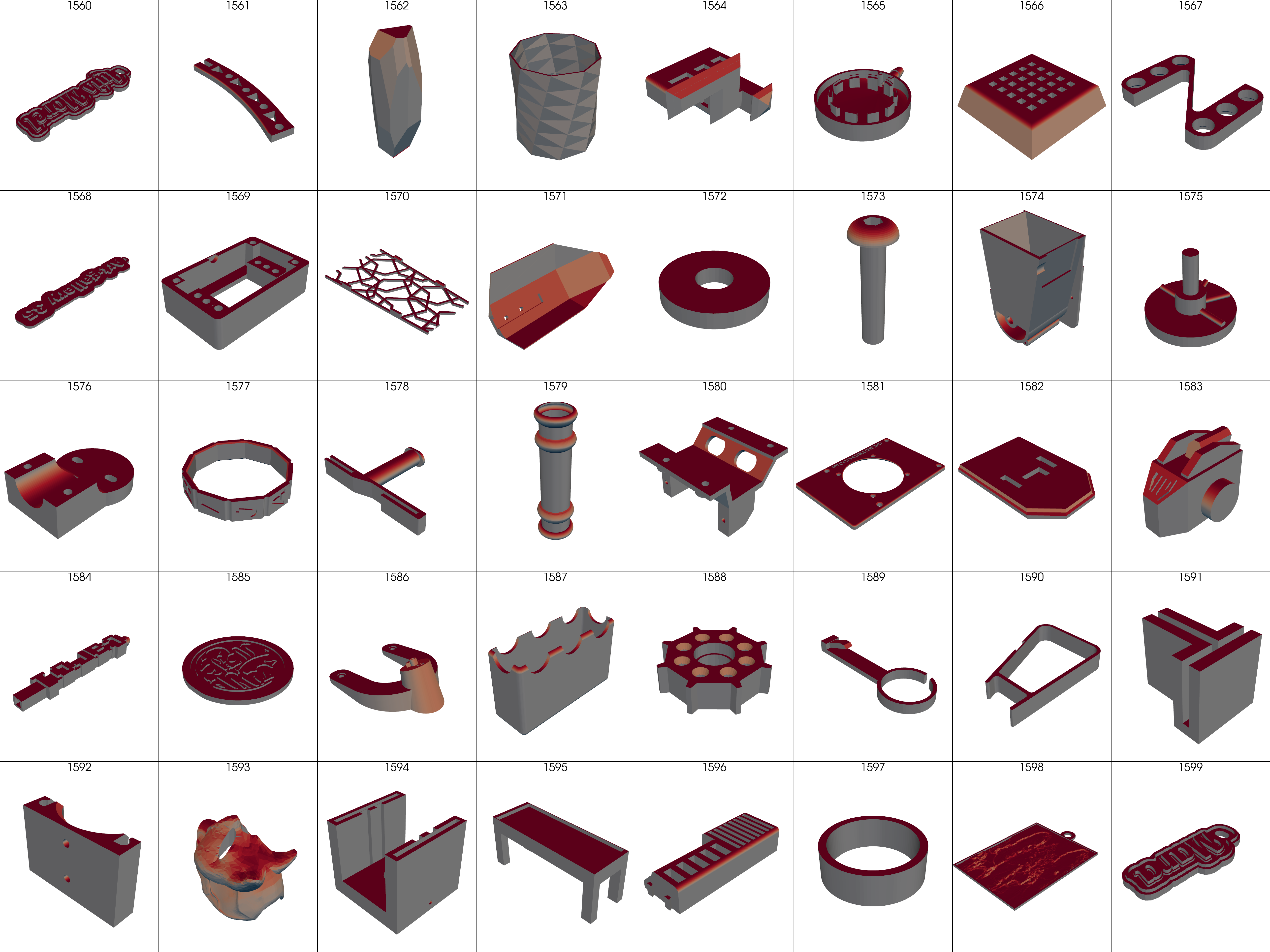
We trained LGM-Aero on AWS as part of the AWS Generative AI Accelerator. After extensive cleaning, filtering and processing of many commercially available datasets of surface meshes, we were able to amass a large training dataset of more than 25 million meshes, comprising more than 100 billion individual mesh elements.
The key steps of the preprocessing were:
- splitting multiple bodied geometries, such as full 3D scenes, into individual geometries;
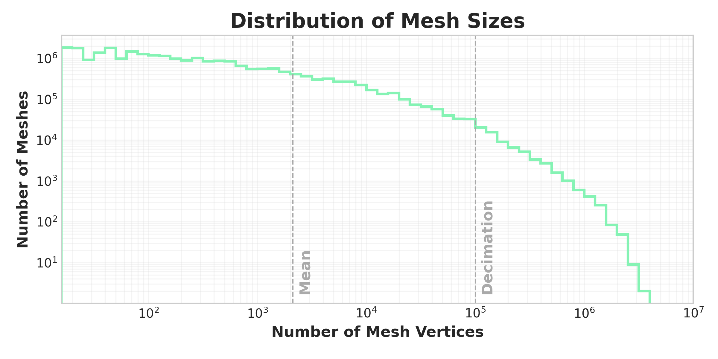
- decimating meshes with more than 100,000 vertices to avoid spending an excessive amount of time training on those meshes;
- ensuring that all meshes were watertight by removing meshes with open edges or whose normals were incorrectly oriented;
All of the data acquisition and preprocessing was carried out on AWS Batch, with files stored on S3 and metadata tracked in DynamoDB.
The final dataset was heavily skewed to coarser and simpler shapes, necessitating a biased sampling strategy during training to ensure that the model was exposed to a more balanced distribution of data. We used the ratio of each object’s volume to the volume of its convex hull to reduce the sampling rate of more convex objects.
Distributing compute
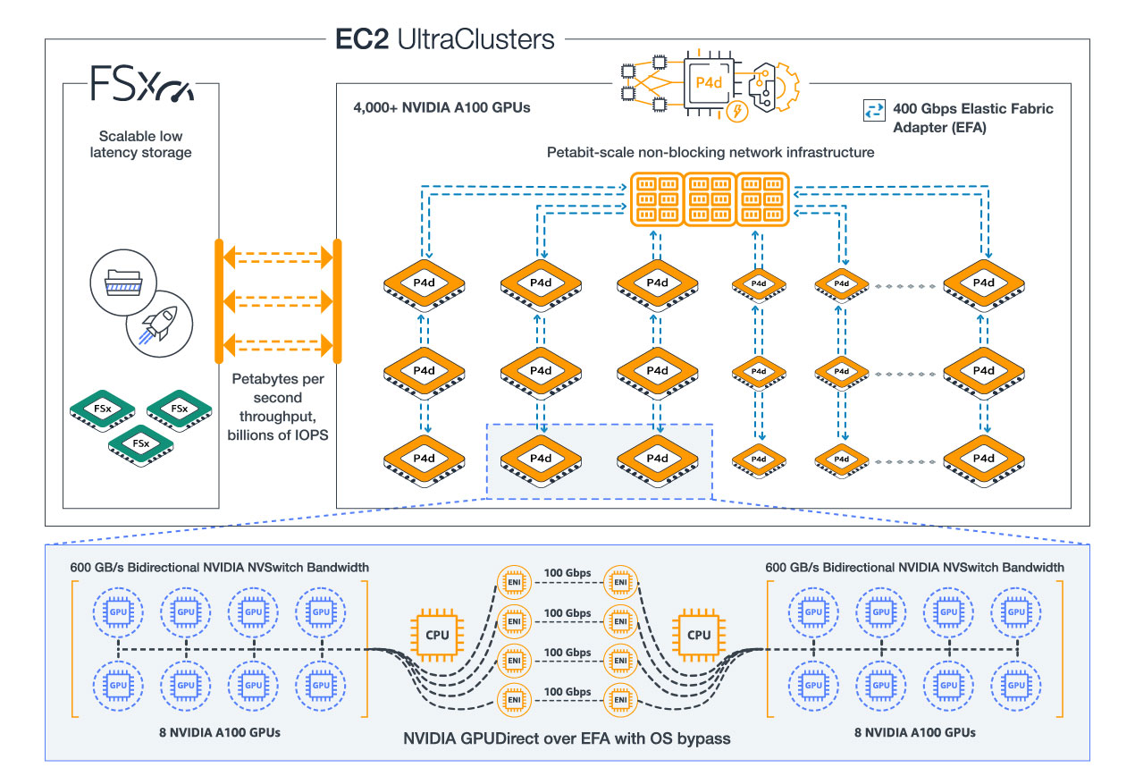
The model was initially trained on 128 Nvidia H100 GPUs (16 AWS P5 instances) for 4 weeks, followed by a further four weeks of training on 64 A100s (8 AWS P4d instances).
Throughout training we employed data-parallelism, where each GPU holds a replica of the model and the training data is partitioned across the processes. The GPUs then act synchronously to process a mini-batch, with the gradients of each mini-batch then averaged across all processes. By ensuring that:
- each model replica begins with the same parameters, \boldsymbol{\theta}_{0};
- each model observes the same gradients at each step, \nabla_{\boldsymbol{\theta}_{t}};
- the optimisation hyperparameters are consistent across processes;
the model replica on each GPU remains consistent during training with parameters at timestep $t$ being described by $\boldsymbol{\theta}{t+1} = \boldsymbol{\theta}{t} - \gamma * \nabla_{\boldsymbol{\theta}_{t}}$ on all GPUs. This approach to distributed/parallel training is known as “mathematically consistent” since the model produced is theoretically equivalent to one trained on a single GPU with an identical batch size.
To improve performance and scalability as we replicated our model across more GPUs, we exploited NCCL with NVLink (intra-machine) and AWS EFA (inter-machine) for fast OS-bypass gradient communication between our GPUs. Similarly, to avoid data I/O bottlenecks and high-latency, we relied on AWS FSx for Lustre (FSx) for distributed file storage mounted to each machine. We found that using FSx, with additional caching mechanisms at the software level, allowed us to achieve disk-like speeds over the network on all our machines simultaneously.
Model structure and losses
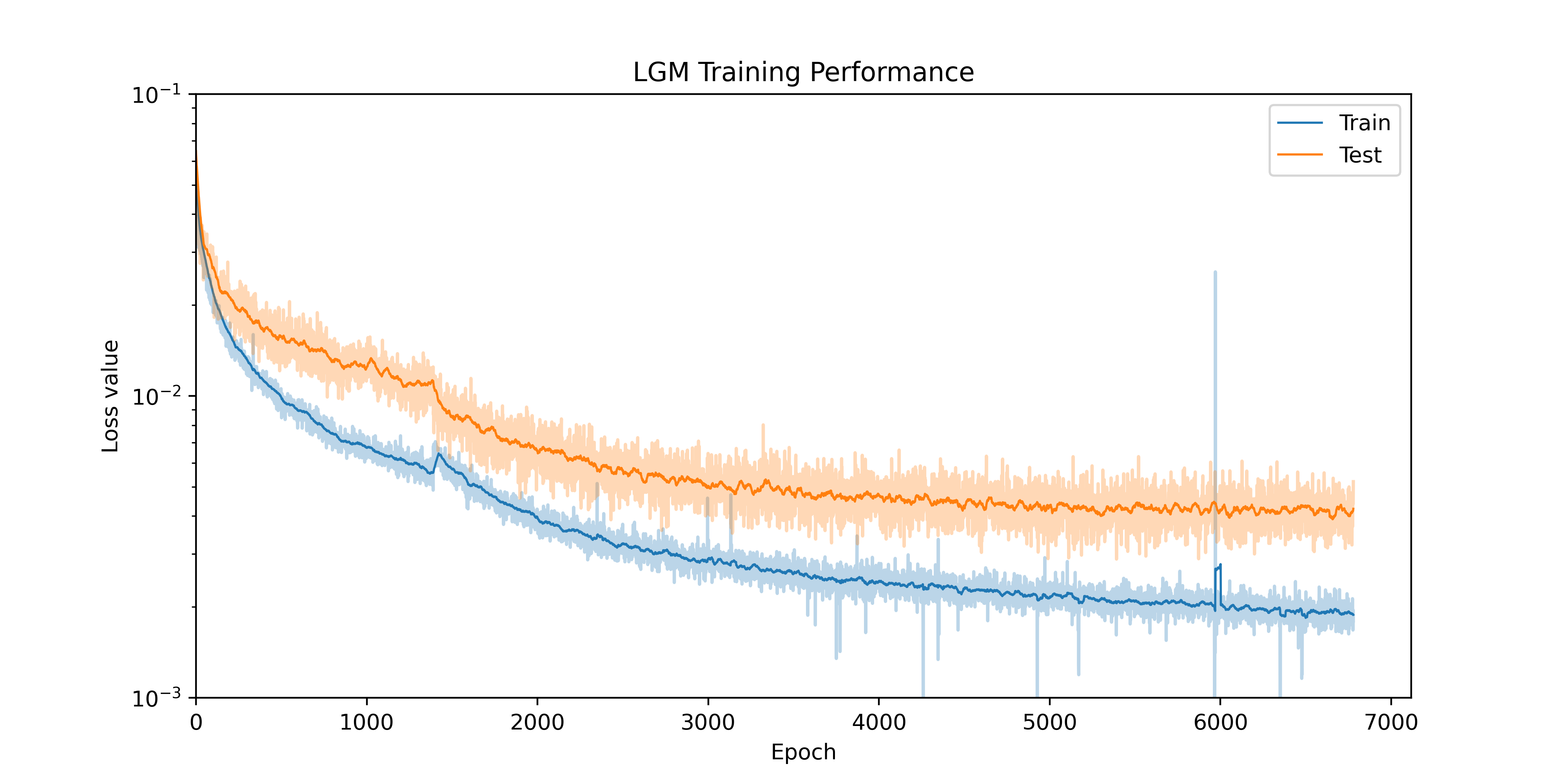
The encoder we used is a diffusion-based neural operator, while the decoder is a modulated residual network. Both model formulation and training procedure is motivated by a probabilistic interpretation and rests on a solid theoretical grounding of approximate inference methods. The encoder outputs a distribution on the latent code of a given mesh, regularised by a Kullback-Leibler divergence with the Gaussian prior, and using Gaussian likelihoods for the reconstruction losses, such that the encoder provides an amortised approximation to the true posterior. Further, losses for geometric consistency were imposed as general priors in the latent space, to promote valid reconstructions with any latent code.
We are preparing a full technical paper describing our methodology and results, and hope to share a preprint early in the new year. In the meantime, check out our live demonstration of this at airplane.physicsx.ai, or book a call with us to talk about how the advanced AI models on our Platform could help transform your engineering process!
Acknowledgements
We would like to thank AWS and the AWS Generative AI Accelerator for support and resources that went towards scaling our latest large geometry model, LGM-Aero.

